CESM-HYCOM GLBb0.08 vs. GLBt0.72
Experimental set-up: HYCOM+CICE+CAM(Atm)+CLM (Land)+RTM (river transports)
-
• GLBt0.72 (gh72): 0.72º (~75km) tripolar grid for Ocean and Ice and a 1.9ºx2.5º grid for the Atmosphere and Land
-
• GLBb0.08 (gh08): 0.08º (~8km) tripolar grid for Ocean and Ice and a 0.47ºx0.63º grid for the Atmosphere and Land
-
• Start from rest with the GDEM4 Climatology for the Ocean component and a constant cover/thickness in the Arctic and Antarctic for the Ice component
-
• HYCOM: 32 hybrid sigma-2 layers, CAM: 26 levels, CICE: 5 categories
-
• No relaxation of sea surface temperature or salinity in HYCOM
-
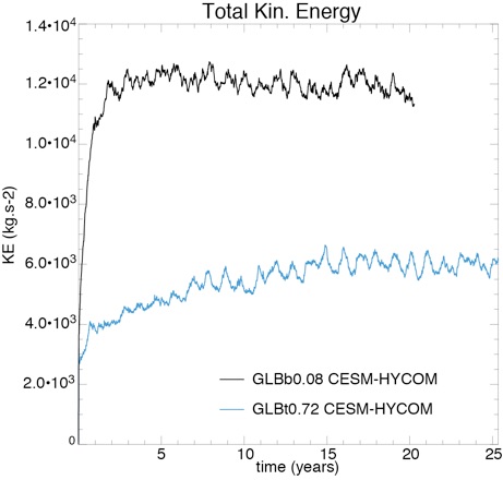
• Simulation of 20 years in high resolution (6 months of computational time) to be compared with 25 years of low resolution (~70 hours).
-
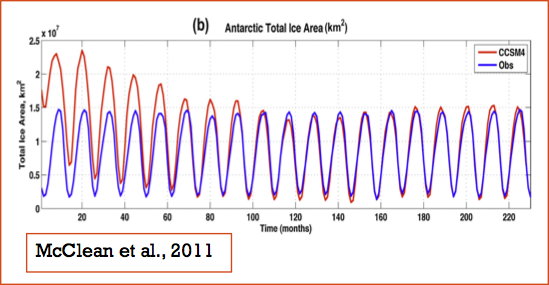
• Evaluation is done against Observations and a 1/10º POP2+CICE+CAM+CLM (CCSM4-POP2) coupled simulation of 20 years described in McClean et al. 2011.
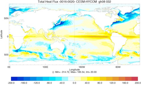
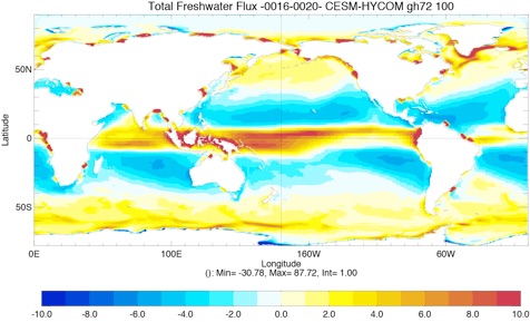
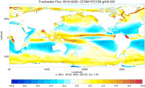
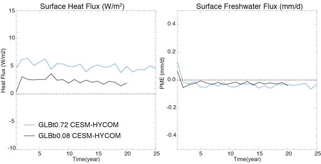
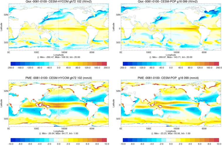
Surface Heat and Freshwater Flux
GLBt0.72
GLBb0.08


Total Kinetic Energy
-
✓ Similar features in GLBt0.72 and GLBb0.08 with strong heat loss over western boundary currents and North Atlantic sub polar gyre, heat gain along the equator.
-
✓ GLBb0.08 colder in North and South Pacific gyres, south Indian Ocean.
-
✓ Similar feature in freshwater flux. Biggest difference in West Pacific.
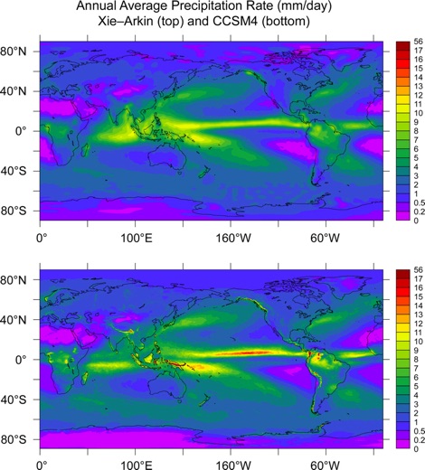
McClean et al. 2011 (CCSM4 1/10º POP2)


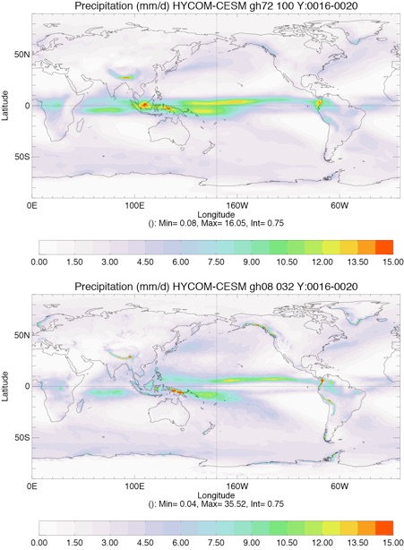
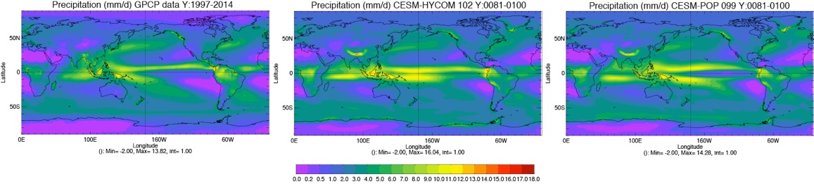
Precipitation (mm/day)
-
✓ Better representation of the precipitation over the Pacific warm pool in high resolution GLBb0.08 and compare well with CCSM4-POP2 simulation with 1/10º grid. (McClean et al. 2011)
-
✓ Lesser intensity of precipitation in HYCOM (GLBb0.08) compare with POP2, but closer to observations.
Evolution of total average Heat and Freshwater Flux
-
✓ Higher surface heat flux in low resolution.
-
✓ Slightly negative freshwater flux for both resolutions.
-
✓ Average Heat FLux:
-
• GLBt0.72: 4.8 ± 0.6 W/m2
-
• GLBb0.08: 1.9 ± 0.3 W/m2
-
✓ Average Freshwater Flux:
-
• GLBt0.72: -0.04 ± 0.01 mm/d
-
• GLBb0.08:-0.03 ± 0.01 mm/d
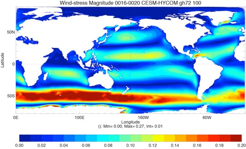
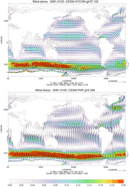
Wind Stress Magnitude

GLBt0.72
GLBb0.08
CORE2 Normal Year on GLBt0.72 grid
-
✓ Over estimation over the Southern Ocean for GLBt0.72 and GLBb0.08.
-
✓ Overestimation over the North Atlantic for GLBb0.08.
-
✓ Better representation of small features in GLBb0.08 compared with CORE2 in South Pacific.
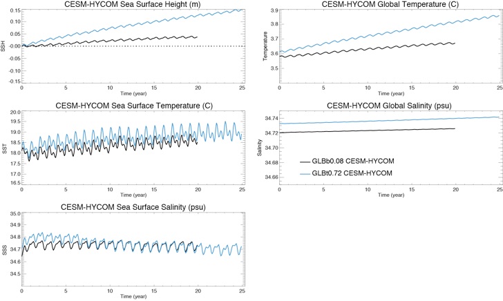
Evolution of T,S,SST,SSS and SSH
-
✓ Global T increases more rapidly in GLBt0.72 due to the bigger heat flux imbalance.
GLBt0.72: + 0.2ºC over 20 years
GLBb0.08: + 0.09ºC over 20 years
-
✓ Slight increase of global S in both GLBt0.72 and GLBb0.08 due to the slight negative averaged freshwater flux.
GLBt0.72: + 0.007 psu over 20 years
GLBb0.08: + 0.005 psu over 20 years
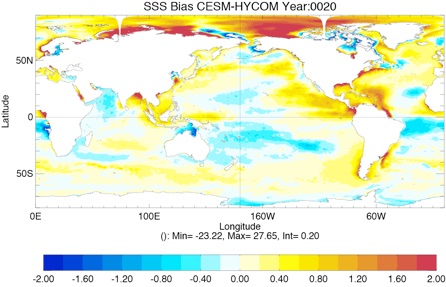
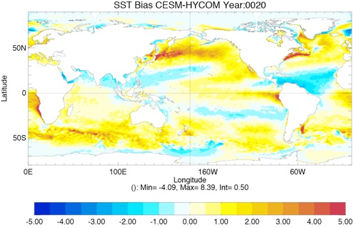
SST and SSS Bias from Climatology
GLBt0.72
GLBb0.08
-
✓ Spatial biases different between GLBt0.72 and GLBb0.08.
-
✓ Less drift in SST overall everywhere in GLBb0.08 compared with GLBt0.72.
-
✓ Less SSS biases in GLBb0.08 overall, except for the Arctic region (ice differences).
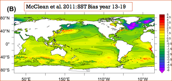
GLBb0.08
-
✓ Similar biases between HYCOM and POP2 except North Atlantic and North Pacific where HYCOM present a positive bias while POP2 presents a negative one .
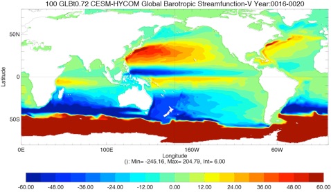
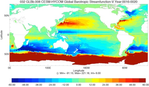
Barotropic Streamfunction
GLBt0.72
GLBb0.08
-
✓ Stronger circulation in the North Atlantic in GLBb0.08.
-
✓ Better representation of the circulation around in the Gulf of Mexico region in GLBb0.08.
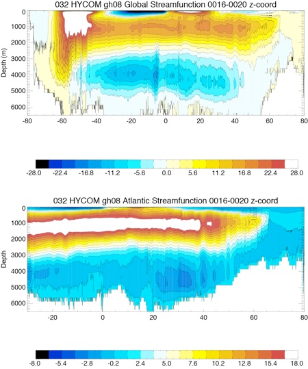
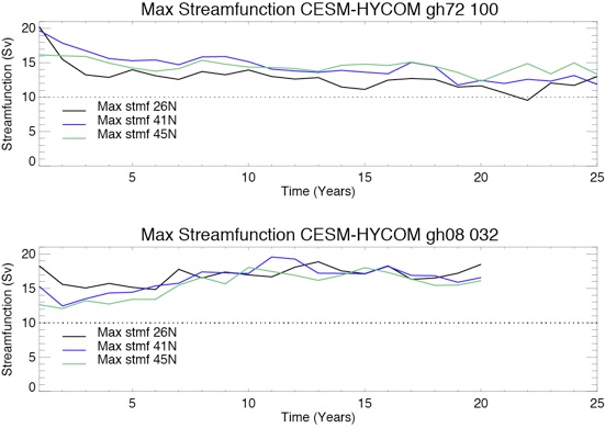
GMOC and AMOC
GLBt0.72
GLBb0.08
GLBb0.08
-
✓ Stronger circulation in in GLBb0.08.

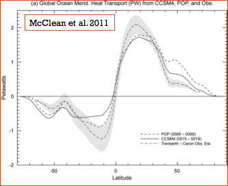
McClean et al. 2011
-
✓ Similar intensity of global circulation in GLBb0.08 compared with CCSM4-POP2 (McClean et al. 2011).
-
✓ Slightly stronger AMOC in GLBb0.08.
-
✓ Decrease of the AMOC in low resolution
-
✓ Increase of the AMOC in high resolution
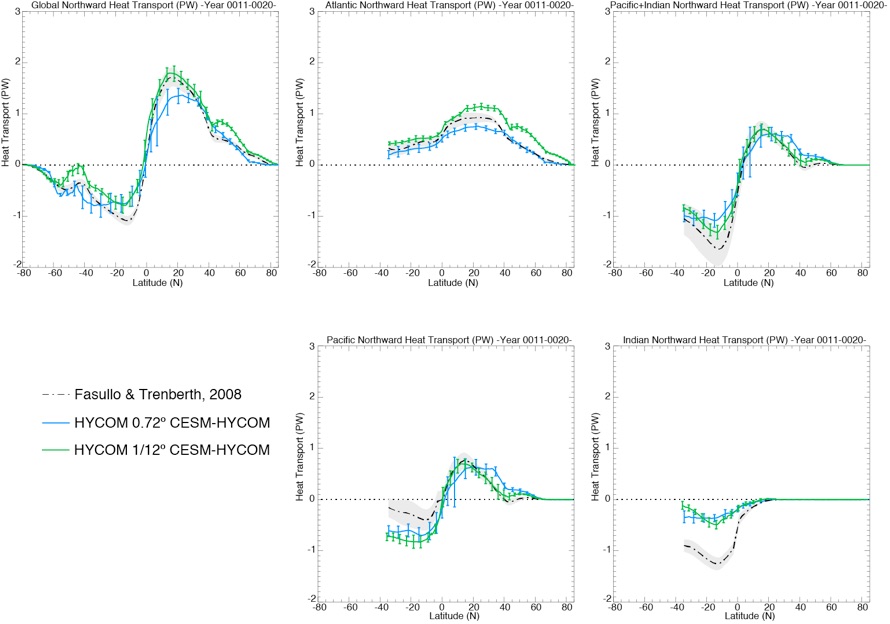
Meridional Heat and Freshwater Transports
-
✓ Stronger heat transports in the mid-latitudes for high resolution GLBb0.08
-
✓ GLB0.08 Heat flux closer to Fasullo & Trenberth (2008).
-
✓ Slightly higher Global Heat transport in GLBb0.08 than in McClean et al. 2011.
-
✓ Similar transport in GLBb0.08 and GLBt0.72 in Indian and Pacific Ocean.
-
✓Higher transport in GLBb0.08 in the Atlantic closer to Trenberth & Fasullo (2017, max of 1.2PW)
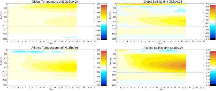
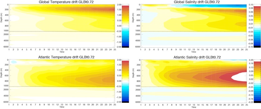
Drift Global T and S
GLBt0.72
GLBb0.08
-
✓ Stronger biases in low resolution
-
✓ Cold/fresh drift at the surface in the Atlantic for GLBb0.08 instead of a warm/salty drift in GLBt0.72


Transports at several sections
-
✓ Stronger transport in GLBt0.72 at the Drake Passage, but transport decreasing.
-
✓ Similar transports at Bering
-
✓ Stronger transport in GLBb0.08 at Florida Straits since most of the transport by-passed the Gulf of Mexico in the low resolution.
-
✓ Stronger Indonesian Throughflow in GLBb0.08 but similar interannual variability
-
✓ GLBb0.08 closer to the observations than GLBt0.72 and CCSM4-POP2
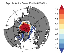
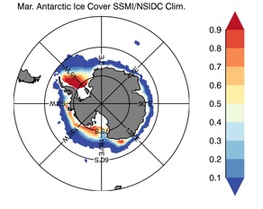
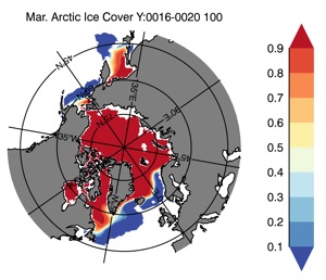
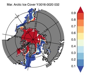
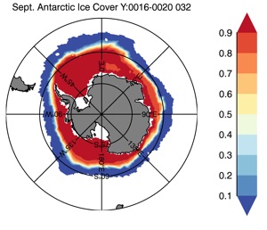
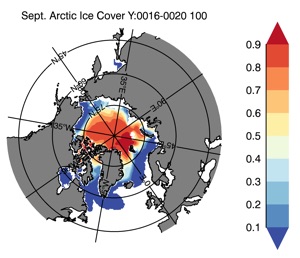
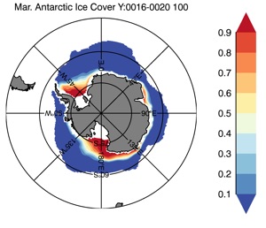
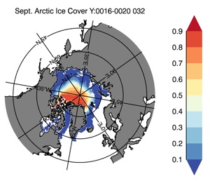
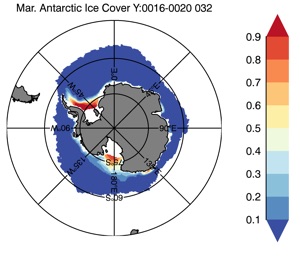
Ice Cover


-
✓ GLBb0.08 ice cover closer to the observations than GLBt0.72 especially in the Arctic.
-
✓ Labrador Sea covered with ice in GLBt0.72 during winter
GLBt0.72
GLBb0.08
SSMI/NSIDC
Winter
SSMI/NSIDC
Summer
GLBt0.72
GLBb0.08
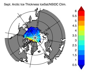
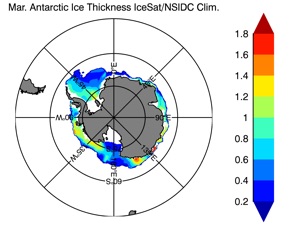
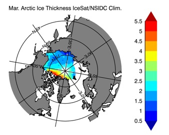
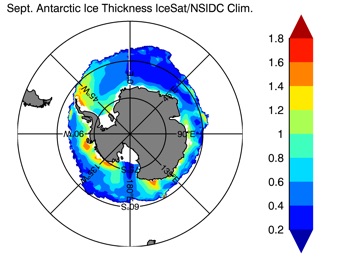
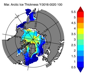
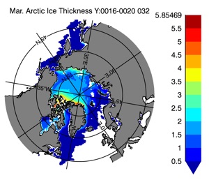
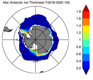
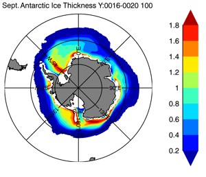
Ice Thickness
Winter
IceSat/NSIDC
GLBt0.72
GLBb0.08
-
✓ Better distribution of Sea Ice thickness in GLBb0.08 than in GLBt0.72.
-
✓ Not enough volume in GLBb0.08 and too much in GLBt0.72.
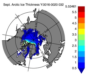
Summer
IceSat/NSIDC
GLBt0.72
GLBb0.08
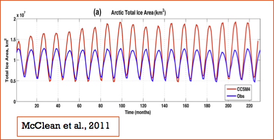
Evolution of ice extent and volume
-
✓ Higher maximum extent in high resolution in Arctic than in the Observations.
-
✓ Linear increase of the sea-ice extent in lower resolution in Arctic.
-
✓ Extent above observations in GLBb0.08 and CCSM4-POP2 in the Arctic but closer to the observations for GLBb0.08.
-
✓Extent below observations in GLBb0.08 and CCSM4-POP2 in the Antarctic but closer to the observations for GLBb0.08.
-
✓ Decrease of the sea-ice volume in GLBb0.08 between year 10 and 20.
GLBt0.72
GLBb0.08
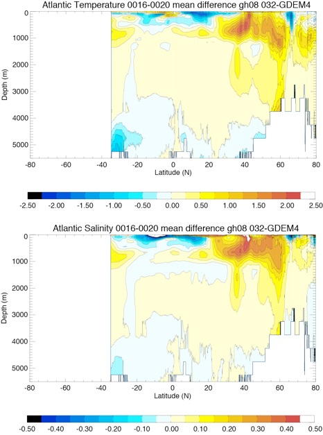
Averaged Meridional Atlantic Section
GLBt0.72
GLBb0.08
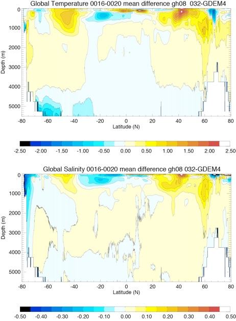
Averaged Meridional Global Section
-
✓ Stronger biases in low resolution
-
✓ Stronger cold/fresh biases in Nordic Seas in low resolution than in high resolution.
-
✓Biases in the Atlantic explain most of the Global biases.


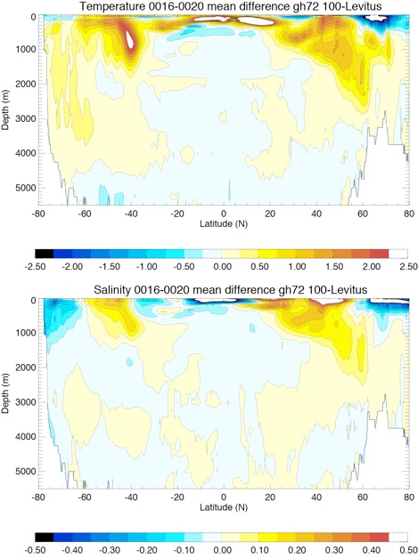


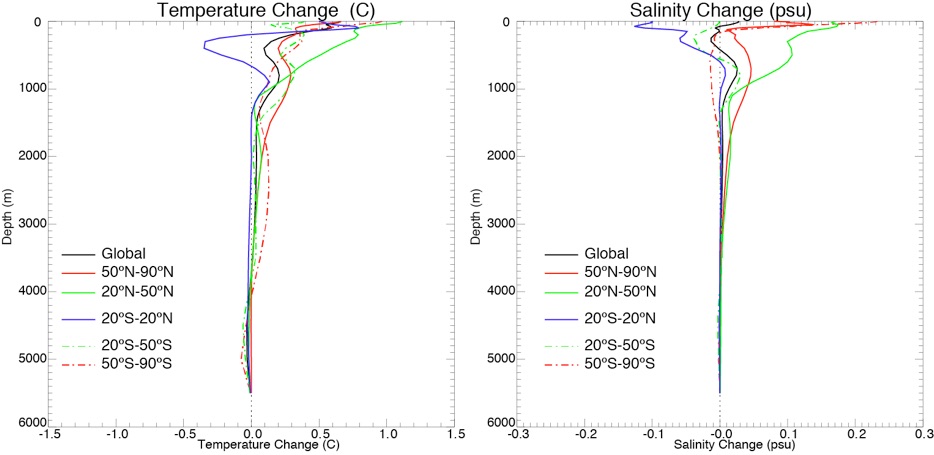
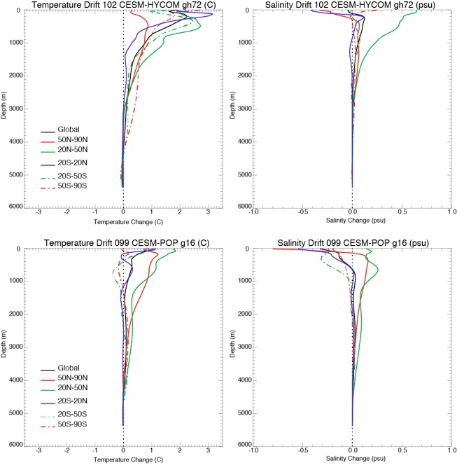
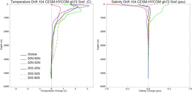
Averaged T and S profile drift per latitudes (Year 0020 - Year 0001)
-
✓ CCSM4 ocean potential temperature (C) (left) and salinity (right) change from model year 19 – model year 1. Red line depicts high latitude regions (50–90), green lines are mid-latitudes (20–50), blue line is the tropics (20S–20N), and black lines are global. Thick and thin lines represent the Northern Hemisphere and Southern Hemispheres, respectively. (McClean et al. 2011)
-
✓Lower global drifts in T and S in HYCOM compared with POP
-
✓Higher drifts at the surface in HYCOM in mid-latitudes, while POP has a maximum around 500m.
-
✓Larger drifts in the tropics in HYCOM

GLBb0.08
GLBt0.72
-
✓ Overall lower drift in GLBb0.08 compared to GLBt0.72
-
✓ Strong positive temperature and negative salinity drift at ~100m and surface respectively in the low resolution in the tropical regions (20ºS-20ºN)
-
✓ Strong Salinity drift in Northern Hemisphere mid-latitude in low resolution
Comparison low resolution experiments -100 years-
Experimental set-up: HYCOM+CICE+CAM(Atm)+CLM (Land)+RTM (river transports)
-
• HYCOM GLBt0.72 (gh72): 0.72º (~75km) tripolar grid for Ocean and Ice and a 1.9ºx2.5º grid for the Atmosphere and Land
-
• POP gx1v6 (g16): 1º (~100km) bipolar grid for Ocean and Ice and a 1.9ºx2.5º grid for the Atmosphere and Land
-
• Start from rest with the Levitus-PHC2 Climatology for the Ocean components and a constant cover/thickness in the Arctic and Antarctic for the Ice component
-
• HYCOM: 32 hybrid sigma-2 layers; POP: 60 z-coord levels, CAM: 26 levels, CICE: 5 categories
-
• No relaxation of sea surface temperature or salinity in HYCOM/POP
-
• Simulation of 100 years in starting from rest.

Outgoing longwave radiation (top of the atmosphere):
CESM-HYCOM f19
CESM-POP f19
Observations
High and low cloud fraction:

Precipitation:
CESM-HYCOM f19
CESM-POP f19
Observations
CESM-HYCOM f19
CESM-POP f19
Observations
Surface heat/freshwater flux and wind stress:
CESM-HYCOM f19
CESM-POP f19
CESM-HYCOM f19
CESM-POP f19
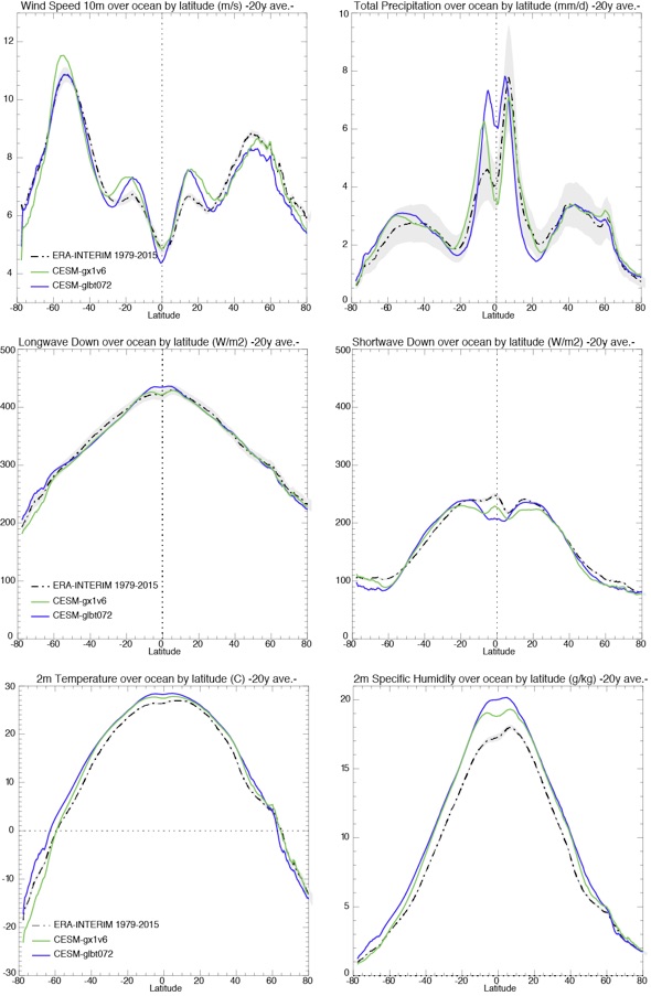
Surface atmospheric variables:

Surface biases:
CESM-HYCOM f19
CESM-POP f19


Salinity
Temperature
Temperature and Salinity evolution:
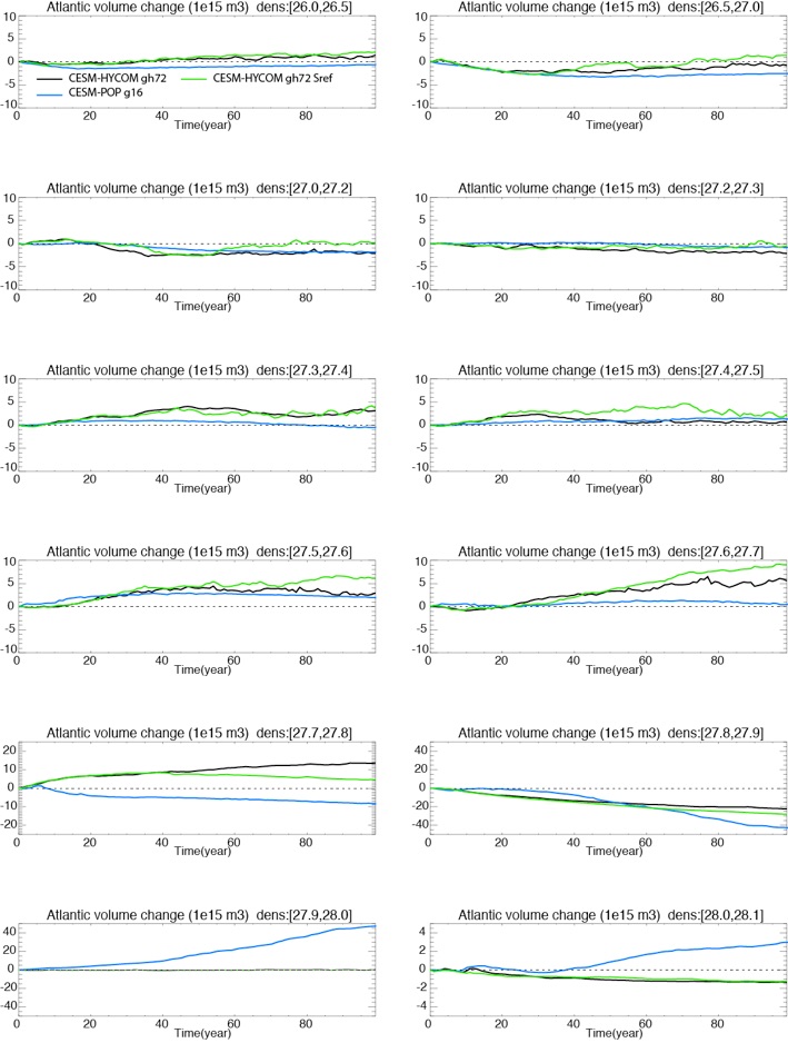
Evolution of water masses in the Atlantic:
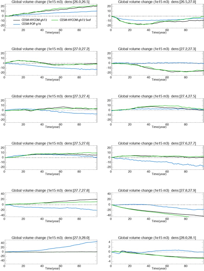
Evolution of water masses total:
Transports at different straits:
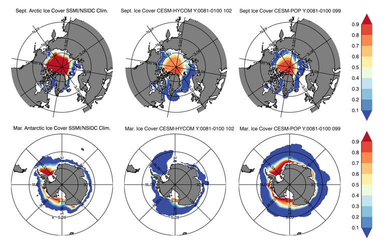
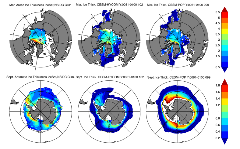
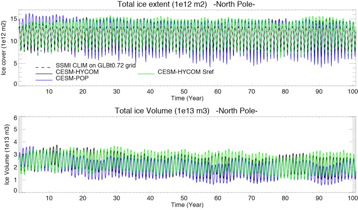
Ice cover and thickness:
CESM-HYCOM f19
CESM-POP f19
Observations
WINTER ICE COVER
CESM-HYCOM f19
CESM-POP f19
Observations
SUMMER ICE COVER
CESM-HYCOM f19
CESM-POP f19
Observations
WINTER ICE THICKNESS
CESM-HYCOM f19
CESM-POP f19
Observations
SUMMER ICE THICKNESS

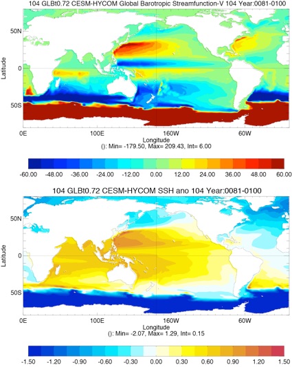
Barotropic Streamfunction and SSH:
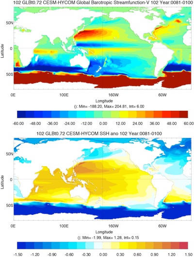
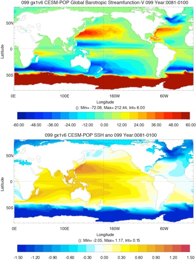
CESM-HYCOM f19
CESM-POP f19
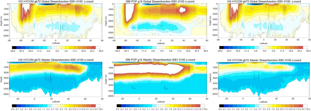
Vertical Streamfunction:
CESM-HYCOM f19
CESM-POP f19
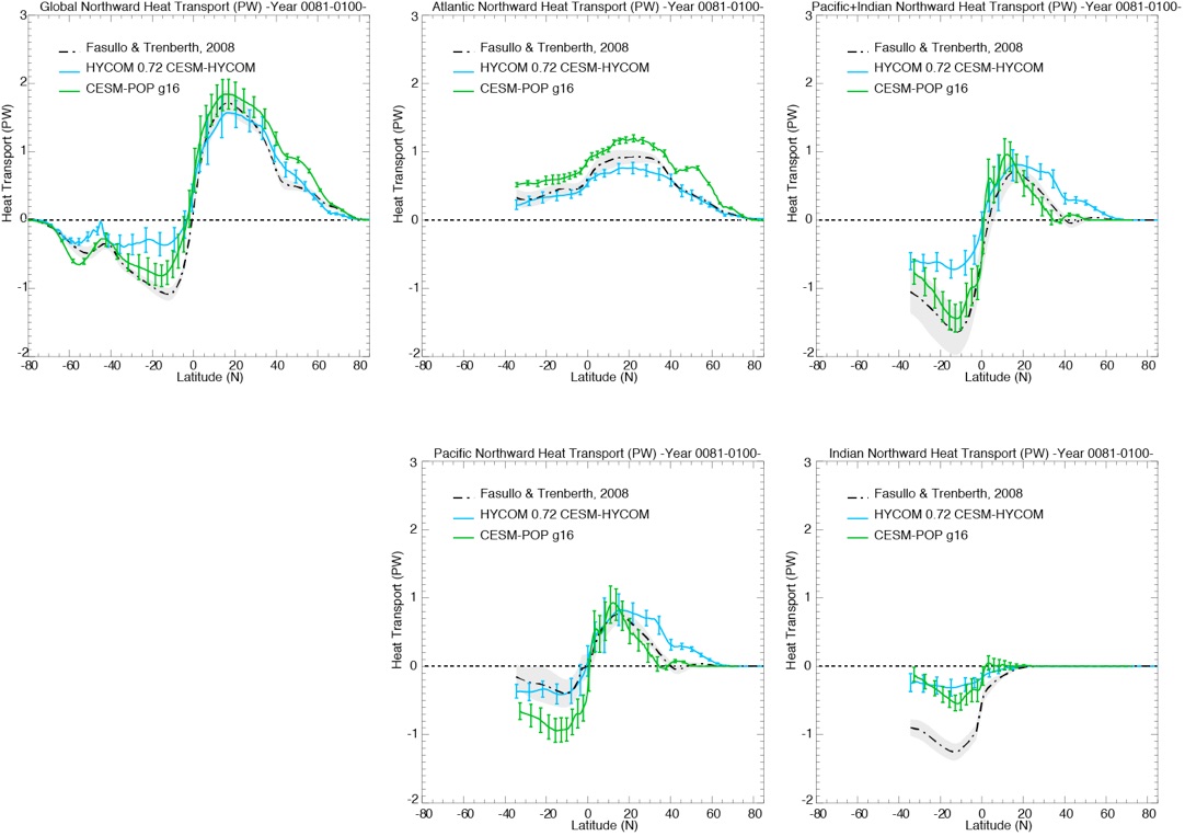
Northward heat and freshwater transports:
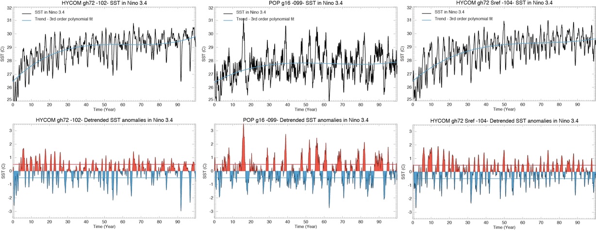
Niño 3.4 index:
-
• Two ITCZ present in HYCOM and POP


-
• Overestimation of Specific Humidity and Temperature
-
• Longwave down and shortwave down close to observations
-
• HYCOM warmer and saltier than POP at the surface
-
• Global surface salinity bias higher than POP mostly because of the polar regions.
-
• Lower global salinity bias when using Sref for salt flux conversion. (Strong freshening of the polar region and Labrador Sea region)
-
• HYCOM global T and S drifts are higher than POP’s even when using Sref for the salt flux.
-
• POP almost stable after 100 years. HYCOM is still showing a strong positive trend.
-
• HYCOM presents a stronger positive drift in temperature at each depth than in POP.
-
• Except in the northern mid-latitude, HYCOM salinity drifts less than POP’s.
-
• Strong surface salinity drift over the northern polar region due to the Sref in salt flux in HYCOM.
(N.B: Drift is average of Years 0081-0100 - Year 0.)
-
• Most of the volume change appears between 27.6 and 27.9 in HYCOM.
-
• HYCOM seems to transform denser water into lighter water (27.8-27.9 into 27.7-27.8)
-
• Most of the volume change appears between 27.7 and 28.0 in POP.
-
• POP seems to transform lighter water into denser water (27.7-27.9 into 27.9-28.0)
-
• As in the Atlantic : Most of the volume change appears between 27.6 and 27.9 in HYCOM.
-
• HYCOM seems to transform denser water into lighter water (27.8-27.9 into 27.7-27.8)
-
• As in the Atlantic: Most of the volume change appears between 27.6 and 28.0 in POP.
-
• POP seems to transform lighter water into denser water (27.6-27.9 into 27.9-28.0)
Obs.: 136.7 +/- 7.8 Sv
Obs.: 0.8 +/- 0.16 Sv
Obs.: -15 Sv
Obs.: -2. +/- 2.7 Sv
-
• HYCOM Drake transport is lower than POP, closer to observations
-
• HYCOM Fram strait is drifting into a positive net northward transport as is usually the behavior of the model at that resolution.
-
• POP Fram strait stays negative and close to the observations.
-
• Transports at Bering and through the Indonesian Throughflow for HYCOM and POP are similar. (lower for Sref)
-
• Probably due to the resolution, HYCOM and POP shows a low transport at the Indonesian Throughflow. (Lower for Sref)
-
• Overestimation of ice cover over the Labrador Sea in HYCOM
-
• POP close to observations
-
• Less ice in the Southern Ocean for HYCOM than in POP.
-
• Overestimation of ice cover in the Arctic in the summer in HYCOM.
-
• POP underestimates the ice cover in the summer.
-
• Less ice in the Southern Ocean for HYCOM than in POP.
-
• Ice thickness higher in HYCOM than POP.
-
• Overestimation of ice thickness in POP and underestimation in HYCOM.
-
• Underestimation of ice thickness in both HYCOM and POP.
-
• Quasi-disappearance of ice in the summer in the Southern Ocean in HYCOM.
-
• Overestimation of ice thickness in the Southern Ocean in POP.
-
• HYCOM’s Ice cover and ice thickness is slowly decreasing over the 100 years of simulation but is stable after year 60.
-
• POP’s ice cover and thickness is stable over the 100 years of simulation.
-
• HYCOM ice cover and thickness is stable over the 100 years.
-
• Less seasonal cycle in HYCOM than in POP.
-
• Ice thickness stabilizes after years 50-60.
-
• North Atlantic gyres stronger in POP than in HYCOM
-
• Vertical Streamfunctions (Global and Atlantic) are stronger in POP than in HYCOM
-
• AMOC too strong in POP (over 20Sv)
-
• AMOC too weak in HYCOM (under 15 SV)
-
• AMOC very weak in HYCOM with Sref because of the freshening of the Labrador Sea region.
-
• As with the streamfunctions, POP presents higher northward heat transports in every basins.
-
• POP is closer to Observations.
-
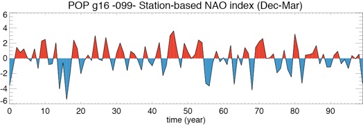
• Higher variability in HYCOM than in POP (more events in HYCOM than in POP).
-
• Stronger and longer events in POP than in HYCOM.
SSH and SSH anomalies
GLBt0.72
GLBb0.08


Station-Based NAO index:


CESM-HYCOM f19 (Sref)


CESM-HYCOM Sref f19
CESM-HYCOM Sref f19

CESM-HYCOM f19
CESM-POP f19
CESM-HYCOM Sref f19
